Use case 4: corner reflector
This section explains how to identify bursts in which the corner reflector (CR), having known geodetic coordinates, is visible, and how to get corrections at CR location.
Notebook setup
[18]:
%matplotlib inline
%load_ext autoreload
%autoreload 2
The autoreload extension is already loaded. To reload it, use:
  %reload_ext autoreload
[19]:
import sys

sys.path.append("../..")
[20]:
import numpy as np
from scipy.interpolate import RegularGridInterpolator
from matplotlib import pyplot as plt
[21]:
import s1etad
from s1etad import Sentinel1Etad
Searching bursts in which the CR is present
Load the S1-ETAD product.
[22]:
filename = (
    "data/"
    "S1A_IW_ETA__AXDV_20230806T211729_20230806T211757_049760_05FBCB_9DD6.SAFE"
)
[23]:
eta = Sentinel1Etad(filename)
The CR position has been chosen to be in the overlap region of different bursts and swaths.
[24]:
from shapely.geometry import Point

lat0 = 32.968825  # 32°58'7.77"N
lon0 = 131.3652  # 131°21'54.72"E
h0 = 304.0

cr = Point(lon0, lat0)
Query for burst covering the CR.
[25]:
selection = eta.query_burst(geometry=cr)
selection
[25]:
| bIndex | pIndex | sIndex | productID | swathID | azimuthTimeMin | azimuthTimeMax | |
|---|---|---|---|---|---|---|---|
| 12 | 8 | 1 | 2 | S1A_IW_SLC__1SDV_20230806T211729_20230806T2117... | IW2 | 2023-08-06 21:17:35.659823903 | 2023-08-06 21:17:38.826979328 |
| 3 | 10 | 1 | 1 | S1A_IW_SLC__1SDV_20230806T211729_20230806T2117... | IW1 | 2023-08-06 21:17:37.478005721 | 2023-08-06 21:17:40.645161146 |
| 13 | 11 | 1 | 2 | S1A_IW_SLC__1SDV_20230806T211729_20230806T2117... | IW2 | 2023-08-06 21:17:38.416422143 | 2023-08-06 21:17:41.612903082 |
Get corrections at CR location
Retrieve the first burst.
[26]:
burst = next(eta.iter_bursts(selection))
Get RADAR coordinates (range and azimuth time) of the CR.
[27]:
tau0, t0 = burst.geodetic_to_radar(lat0, lon0, h0)
tau0, t0
[27]:
(array([0.00031842]), array([9.42706234]))
Get image coordinates (line and sample) of the CR.
NOTE: image coordinates area floating point numbers including pixel fractions.
[28]:
line, sample = burst.radar_to_image(t0, tau0)
print(f"Line {line} of {burst.lines}, sample {sample} of {burst.samples}.")
Line [101.46282565] of 109, sample [10.58569122] of 478.
Get the correction.
[29]:
correction = burst.get_correction(s1etad.ECorrectionType.SUM, meter=True)
data = correction["x"]  # summ of corrections in the range direction
Interpolate the correction at the specified RADAR coordinates (tau0, t0).
[30]:
azimuth_time, range_time = burst.get_burst_grid()

interpolator = RegularGridInterpolator((range_time, azimuth_time), data.T)

value_at_radar_coordinates = interpolator((tau0, t0))

print(
    "The correction value at RADAR coordinates "
    f"(tau0, t0) = ({tau0}, {t0}) is {value_at_radar_coordinates}"
)
The correction value at RADAR coordinates (tau0, t0) = ([0.00031842], [9.42706234]) is [3.1933344]
Interpolate the correction at the specified image coordinates (line, sample).
[31]:
xaxis = np.arange(burst.samples)
yaxis = np.arange(burst.lines)

interpolator = RegularGridInterpolator((xaxis, yaxis), data.T)

value_at_image_coordinates = interpolator((sample, line))

print(
    "The correction value at image coordinates "
    f"(sample, line) = ({sample}, {line}) is {value_at_image_coordinates}"
)
The correction value at image coordinates (sample, line) = ([10.58569122], [101.46282565]) is [3.1933344]
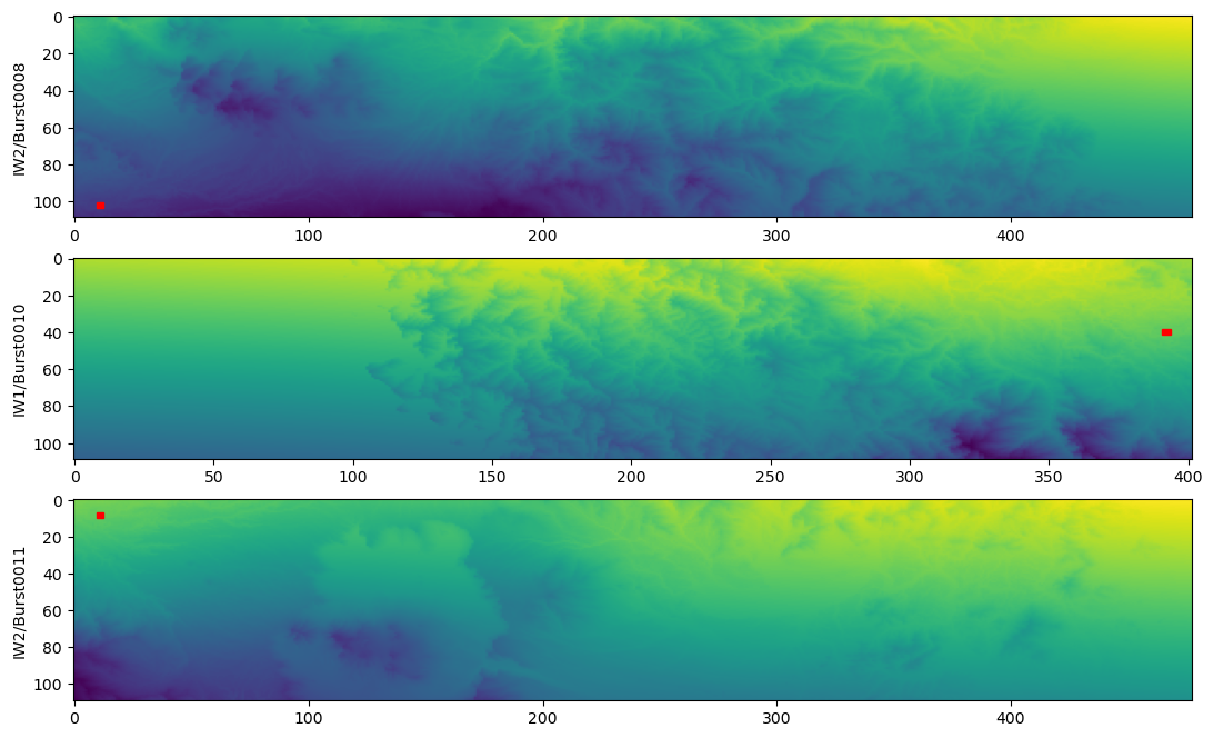
Putting all together
[32]:
from matplotlib.patches import Rectangle

fig, ax = plt.subplots(nrows=len(selection), ncols=1, figsize=[13, 8])

if len(selection) < 2:
    ax = [ax]

for loop, burst in enumerate(eta.iter_bursts(selection)):
    # get RADAR and image coordinates
    tau0, t0 = burst.geodetic_to_radar(lat0, lon0)
    line0, sample0 = burst.radar_to_image(t0, tau0)
    print(
        "xy  ",
        burst.swath_id,
        burst.burst_index,
        line0,
        sample0,
        burst.radar_to_geodetic(tau0, t0),
    )
    print(
        "time",
        burst.swath_id,
        burst.burst_index,
        tau0,
        t0,
        burst.radar_to_geodetic(tau0, t0),
    )

    # correction
    cor = burst.get_correction(s1etad.ECorrectionType.SUM, meter="True")

    ax[loop].imshow(cor["x"], aspect="auto")
    ax[loop].set_ylabel(f"{burst.swath_id}/{burst.burst_id}")
    rec_half_size = 1
    p = Rectangle(
        (sample0 - rec_half_size, line0 - rec_half_size),
        width=rec_half_size * 2 + 1,
        height=rec_half_size * 2 + 1,
        color="red",
        fill=True,
    )
    ax[loop].add_patch(p)

    # get the range and azimuth time axes
    azimuth_time, range_time = burst.get_burst_grid()

    # interpolate at the desired working (RADAR) coordinates
    f_t = RegularGridInterpolator((range_time, azimuth_time), cor["x"].T)

    # get the image (lines and samples) axes
    yaxis = np.arange(azimuth_time.size)
    xaxis = np.arange(range_time.size)

    # interpolate at the desired working (image) coordinates
    f_ij = RegularGridInterpolator((xaxis, yaxis), cor["x"].T)

    print(
        f"Interpolation by array coordinate {f_ij((sample0, line0))} or "
        f"time {f_t((tau0, t0))} should be the same"
    )
    print(
        f"The total correction at lat/lon {lat0, lon0} is "
        f" {f_ij((sample0, line0))} m in range"
    )
    print()
xy   IW2 8 [101.46282565] [10.58569122] (array([32.968825]), array([131.3652]), array([331.88771595]))
time IW2 8 [0.00031842] [9.42706234] (array([32.968825]), array([131.3652]), array([331.88771595]))
Interpolation by array coordinate [3.1933344] or time [3.1933344] should be the same
The total correction at lat/lon (32.968825, 131.3652) is  [3.1933344] m in range

xy   IW1 10 [39.4628219] [391.58561982] (array([32.968825]), array([131.3652]), array([331.8869369]))
time IW1 10 [0.00031842] [9.42706223] (array([32.968825]), array([131.3652]), array([331.8869369]))
Interpolation by array coordinate [3.69389987] or time [3.69389987] should be the same
The total correction at lat/lon (32.968825, 131.3652) is  [3.69389987] m in range

xy   IW2 11 [7.46282484] [10.58550757] (array([32.968825]), array([131.3652]), array([331.88500572]))
time IW2 11 [0.00031842] [9.42706231] (array([32.968825]), array([131.3652]), array([331.88500572]))
Interpolation by array coordinate [3.98766172] or time [3.98766172] should be the same
The total correction at lat/lon (32.968825, 131.3652) is  [3.98766172] m in range
[33]:
burst.radar_to_geodetic(tau0, t0)
[33]:
(array([32.968825]), array([131.3652]), array([331.88500572]))
[34]:
cor
[34]:
{'x': array([[4.05822451, 4.0607732 , 4.05306037, ..., 4.39878131, 4.39897736,
         4.39914722],
        [4.0458467 , 4.05001574, 4.0482936 , ..., 4.3906227 , 4.39040733,
         4.39159507],
        [4.0477595 , 4.03773197, 4.03714374, ..., 4.38187025, 4.38249812,
         4.38309924],
        ...,
        [2.67421528, 2.68387344, 2.69863569, ..., 3.54058138, 3.5411553 ,
         3.54173328],
        [2.65510669, 2.67399737, 2.69620666, ..., 3.53260976, 3.53318217,
         3.53376219],
        [2.64196745, 2.65870343, 2.67874309, ..., 3.52462466, 3.52520104,
         3.52578767]], shape=(110, 478)),
 'y': array([[-1.37837932, -1.37512413, -1.39237992, ..., -2.14400831,
         -2.1436258 , -2.14326606],
        [-1.39020902, -1.38386951, -1.38911398, ..., -2.15940761,
         -2.15987731, -2.1576086 ],
        [-1.37411534, -1.39526828, -1.39826819, ..., -2.17580657,
         -2.17471202, -2.17364075],
        ...,
        [-0.35608611, -0.38188736, -0.41922822, ..., -3.07435376,
         -3.08063787, -3.08695525],
        [-0.30717491, -0.3551246 , -0.41032683, ..., -3.07630146,
         -3.08265162, -3.08903569],
        [-0.27148865, -0.3152747 , -0.36651941, ..., -3.07812449,
         -3.08454058, -3.09099141]], shape=(110, 478)),
 'unit': 'm',
 'name': 'sum'}