Use case 3: retrieving footprints
Notebook setup
[1]:
%matplotlib inline
%load_ext autoreload
%autoreload 2
[2]:
import sys

sys.path.append("../..")
[3]:
import numpy as np
import matplotlib.pyplot as plt
[4]:
from s1etad import Sentinel1Etad
Open the dataset
[5]:
filename = (
    "data/"
    "S1A_IW_ETA__AXDV_20230806T211729_20230806T211757_049760_05FBCB_9DD6.SAFE"
)
[6]:
eta = Sentinel1Etad(filename)
[7]:
eta
[7]:
Sentinel1Etad("data/S1A_IW_ETA__AXDV_20230806T211729_20230806T211757_049760_05FBCB_9DD6.SAFE")  # 0x78520a2dd7f0
Number of Sentinel-1 slices: 1
Sentinel-1 products list:
  S1A_IW_SLC__1SDV_20230806T211729_20230806T211757_049760_05FBCB_BC56.SAFE
Number of swaths: 3
Swath list: IW1, IW2, IW3
Azimuth time:
  min: 2023-08-06 21:17:29.208211
  max: 2023-08-06 21:17:57.184751
Range time:
  min: 0.0053335639608434815
  max: 0.006389868212274445
Grid sampling:
  x: 8.131672451354599e-07
  y: 0.02932551319648094
  unit: s
Grid spacing:
  x: 200.0
  y: 200.0
  unit: m
Processing settings:
  troposphericDelayCorrection: True
  troposphericDelayCorrectionGradient: True
  ionosphericDelayCorrection: True
  solidEarthTideCorrection: True
  oceanTidalLoadingCorrection: True
  bistaticAzimuthCorrection: True
  dopplerShiftRangeCorrection: True
  FMMismatchAzimuthCorrection: True
Helpers
[8]:
import cartopy.crs as ccrs
from matplotlib import patches as mpatches
from shapely.geometry import MultiPolygon


def tile_extent(poly, margin=2):
    bounding_box = list(poly.bounds)
    bounding_box[1:3] = bounding_box[2:0:-1]
    return np.asarray(bounding_box) + [-margin, margin, -margin, margin]
Select bursts
[9]:
import dateutil

first_time = dateutil.parser.parse("2023-08-06T21:17:29.240420")
selection = eta.query_burst(first_time=first_time)
Get footprints of the selected bursts
[10]:
polys = eta.get_footprint(selection=selection)
[11]:
polys
[11]:

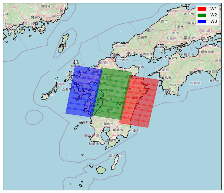
Plot footprints
[12]:
fig = plt.figure(figsize=[10, 8])
ax = fig.add_subplot(1, 1, 1, projection=ccrs.PlateCarree())
ax.set_extent(tile_extent(MultiPolygon(polys)))

# Put a background image on for nice sea rendering.
OFFLINE = False
if OFFLINE:
    import cartopy.feature as cfeature

    ax.stock_img()
    ax.add_feature(cfeature.LAND)
    ax.add_feature(cfeature.COASTLINE)
else:
    import cartopy.io.img_tiles as cimgt

    # stamen_terrain = cimgt.Stamen("terrain-background")# need cartopy >= 0.17
    img = cimgt.OSM()
    ax.add_image(img, 7)  # up to 10
    ax.coastlines()

# plot footprints of all selected burst
# ax.add_geometries(polys, crs=ccrs.PlateCarree(), alpha=0.8)

# get the footprints of each swath and plot them with different colors
items = []
for swath, color in zip(eta, ["red", "green", "blue"], strict=False):
    polys = swath.get_footprint(selection=selection)
    item = ax.add_geometries(
        polys, crs=ccrs.PlateCarree(), alpha=0.5, color=color
    )
    items.append(item)

handles = [
    mpatches.Patch(color=color, label=label)
    for color, label in zip(
        ["red", "green", "blue"], eta.swath_list, strict=False
    )
]
plt.legend(handles=handles)
[12]:
<matplotlib.legend.Legend at 0x7851f7dd0050>