Use case 2: retrieving the corrections
Notebook setup
[1]:
%matplotlib inline
%load_ext autoreload
%autoreload 2
[2]:
import sys
sys.path.append('../..')
[3]:
import numpy as np
import matplotlib.pyplot as plt
[4]:
import s1etad
from s1etad import Sentinel1Etad, ECorrectionType
Open the dataset
[5]:
filename = '../../sample-products/S1B_IW_ETA__AXDH_20200127T113414_20200127T113858_020002_025D72_0096.SAFE'
[6]:
eta = Sentinel1Etad(filename)
[7]:
swath = eta['IW1']
[8]:
burst = swath[1]
[9]:
burst
[9]:
Sentinel1EtadBurst("/IW1/Burst0001")  0x7f87a22a6790
Swaths ID: IW1
Burst index: 1
Shape: (111, 403)
Sampling start:
  x: 0.0
  y: 0.0
  units: s
Sampling:
  x: 8.081406101630269e-07
  y: 0.028777788199999974
  units: s
Get corrections
The Sentinel1EtadBurst class allows to access the netcdf product to retrieve the corrections burst by burst.
The recommended way to retrieve a correction is:
s1etad.Sentinel1EtadBurst.get_correction(name, set_auto_mask=False,
                                         transpose=True, meter=False)
Available correction types are:
[10]:
s1etad.ECorrectionType.__members__
[10]:
mappingproxy({'TROPOSPHERIC': <ECorrectionType.TROPOSPHERIC: 'tropospheric'>,
              'IONOSPHERIC': <ECorrectionType.IONOSPHERIC: 'ionospheric'>,
              'GEODETIC': <ECorrectionType.GEODETIC: 'geodetic'>,
              'BISTATIC': <ECorrectionType.BISTATIC: 'bistatic'>,
              'DOPPLER': <ECorrectionType.DOPPLER: 'doppler'>,
              'FMRATE': <ECorrectionType.FMRATE: 'fmrate'>,
              'SUM': <ECorrectionType.SUM: 'sum'>})
Example:
[11]:
# correction = burst.get_correction('ionospheric')
#
# or equivalently
correction = burst.get_correction(s1etad.ECorrectionType.IONOSPHERIC, meter=True)
correction.keys()
[11]:
dict_keys(['x', 'unit', 'name'])
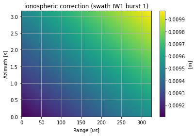
[12]:
az, rg = burst.get_burst_grid()
extent = [rg[0]*1e6, rg[-1]*1e6, az[0], az[-1]]

plt.figure()
plt.imshow(correction['x'], extent=extent, aspect='auto')
plt.xlabel('Range [$\mu s$]')
plt.ylabel('Azimuth [s]')
plt.grid()
plt.colorbar().set_label(f'[{correction["unit"]}]')
plt.title(f'{correction["name"]} correction (swath {burst.swath_id} burst {burst.burst_index})')
[12]:
Text(0.5, 1.0, 'ionospheric correction (swath IW1 burst 1)')
Retrieving merged corrections
The Sentinel1Etad and Sentinel1EtadSwath classes provides methods to retrieve a specific correction for multiple bursts merged together for easy representation purposes.
NOTE: the current implementation uses a very simple algorithm that iterates over selected bursts and stitches correction data together. In overlapping regions new data simply overwrite the old ones. This is an easy algorithm and perfectly correct for atmospheric and geodetic correction. It is, instead, sub-optimal for system corrections (bi-static, Doppler, FM Rate) which have different values in overlapping regions.
First select the bursts
[13]:
import dateutil.parser

first_time = dateutil.parser.parse('2020-01-27T11:34:31.022825')
last_time =  dateutil.parser.parse('2020-01-27T11:34:56.260946')

product_name = 'S1B_IW_SLC__1ADH_20200127T113414_20200127T113444_020002_025D72_FD42.SAFE'

# query the catalogue for a subset of the swaths
df = eta.query_burst(first_time=first_time, last_time=last_time, product_name=product_name)

# df = df[df.bIndex != 13]   # exclude burst n. 13 (IW1)) to test extended selection capabilities
# df = df[df.bIndex != 17]   # exclude burst n. 17 (IW2)) to test extended selection capabilities
# df = df[df.bIndex != 15]   # exclude burst n. 17 (IW3)) to test extended selection capabilities
Common variables
[14]:
from scipy import constants

dy = eta.grid_spacing['y']
dx = eta.grid_sampling['x'] * constants.c / 2
nswaths = len(df.swathID.unique())
vg = eta.grid_spacing['y'] / eta.grid_sampling['y']
vmin = 2.5
vmax = 3.5
to_km = 1. / 1000
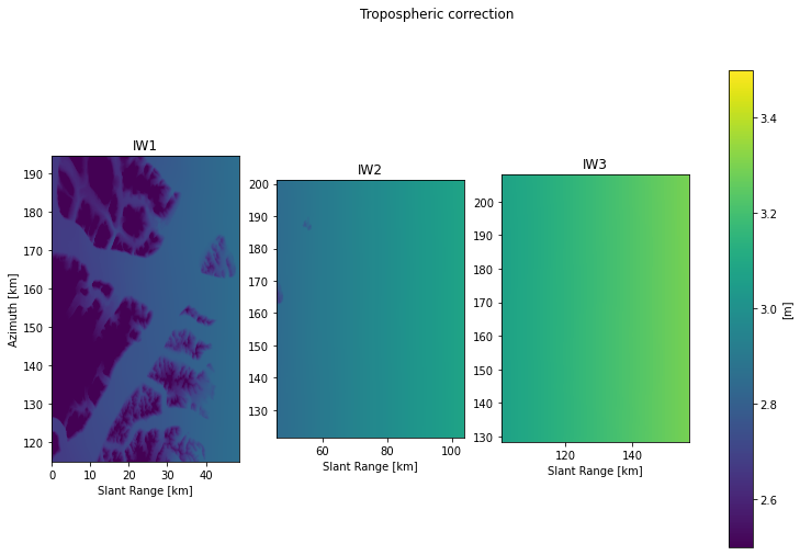
Iterate on swath to get de-bursted data (selected burst merged together)
[15]:
fig, ax = plt.subplots(nrows=1, ncols=nswaths, figsize=[13, 8])
for idx, swath in enumerate(eta.iter_swaths(df)):
    merged_correction = swath.merge_correction(ECorrectionType.TROPOSPHERIC,
                                               selection=df, meter=True)
    merged_correction_data = merged_correction['x']

    ysize, xsize = merged_correction_data.shape
    x0 = merged_correction['first_slant_range_time'] * constants.c / 2  # [m]
    y0 = merged_correction['first_azimuth_time'] * vg                   # [m]
    x_axis = (x0 + np.arange(xsize) * dx) * to_km
    y_axis = (y0 + np.arange(ysize) * dy) * to_km

    extent=[x_axis[0], x_axis[-1], y_axis[0], y_axis[-1]]
    im = ax[idx].imshow(merged_correction_data, origin='lower', extent=extent,
                        vmin=vmin, vmax=vmax, aspect='equal')
    ax[idx].set_title(swath.swath_id)
    ax[idx].set_xlabel('Slant Range [km]')

ax[0].set_ylabel('Azimuth [km]')

name = merged_correction['name']
unit = merged_correction['unit']

fig.suptitle(f'{name.title()} correction')
fig.colorbar(im, ax=ax[:].tolist(), label=f'[{unit}]')
[15]:
<matplotlib.colorbar.Colorbar at 0x7f87a4abc310>
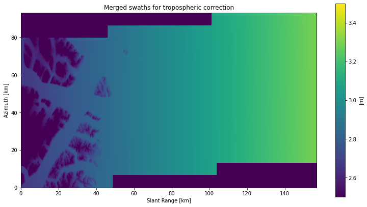
Get merged swaths
[16]:
fig, ax = plt.subplots(figsize=[13, 7])
merged_correction = eta.merge_correction(ECorrectionType.TROPOSPHERIC,
                                         selection=df, meter=True)
merged_correction_data = merged_correction['x']

ysize, xsize = merged_correction_data.shape
x_axis = np.arange(xsize) * dx * to_km
y_axis = np.arange(ysize) * dy * to_km

extent=[x_axis[0], x_axis[-1], y_axis[0], y_axis[-1]]
im = ax.imshow(merged_correction_data, origin='lower', extent=extent,
               vmin=vmin, vmax=vmax, aspect='equal')

ax.set_xlabel('Slant Range [km]')
ax.set_ylabel('Azimuth [km]')

name = merged_correction['name']
unit = merged_correction['unit']

ax.set_title(f'Merged swaths for {name} correction')
fig.colorbar(im, ax=ax, label=f'[{unit}]')
[16]:
<matplotlib.colorbar.Colorbar at 0x7f878fd56f50>