[1]:
%matplotlib inline

import numpy as np
from scipy import constants
import matplotlib.pyplot as plt
[2]:
%load_ext autoreload
%autoreload 2

import s1etad
from s1etad import Sentinel1Etad, ECorrectionType
s1etad Python module: basic usage
Sentinel1Etad product
[3]:
filename = 'test/S1B_IW_ETA__AXDV_20190805T162509_20190805T162536_017453_020D3A_____.SAFE'
eta_ = Sentinel1Etad(filename)
[4]:
eta_
[4]:
Sentinel1Etad("test/S1B_IW_ETA__AXDV_20190805T162509_20190805T162536_017453_020D3A_____.SAFE")  # 0x7f8322328950
Sentinel-1 products list:
  S1B_IW_SLC__1ADV_20190805T162509_20190805T162536_017453_020D3A_A857.SAFE
Number of swaths: 3
Swath list: IW1, IW2, IW3
Grid sampling:
  x: 8.081406101630269e-07
  y: 0.028777788199999974
  unit: s
Grid spacing:
  x: 200.0
  y: 200.0
  unit: m
Processing settings:
  troposphericDelayCorrection: True
  ionosphericDelayCorrection: True
  solidEarthTideCorrection: True
  bistaticAzimuthCorrection: True
  dopplerShiftRangeCorrection: True
  FMMismatchAzimuthCorrection: True
Check which corrections have been enabled
[5]:
eta_.processing_setting()
[5]:
{'troposphericDelayCorrection': True,
 'ionosphericDelayCorrection': True,
 'solidEarthTideCorrection': True,
 'bistaticAzimuthCorrection': True,
 'dopplerShiftRangeCorrection': True,
 'FMMismatchAzimuthCorrection': True}
The burst catalogue
It is a pandas dataframe to allow easy filtering.
See also use cases in the “Use case 1: Selecting the bursts” section for a more complete explaination on the burst catalogue and the query mechanism.
[6]:
eta_.burst_catalogue.head()
[6]:
| bIndex | pIndex | sIndex | productID | swathID | azimuthTimeMin | azimuthTimeMax | |
|---|---|---|---|---|---|---|---|
| 0 | 1 | 1 | 1 | S1B_IW_SLC__1ADV_20190805T162509_20190805T1625... | IW1 | 2019-08-05 16:25:09.836779 | 2019-08-05 16:25:13.002336 |
| 1 | 4 | 1 | 1 | S1B_IW_SLC__1ADV_20190805T162509_20190805T1625... | IW1 | 2019-08-05 16:25:12.570669 | 2019-08-05 16:25:15.736226 |
| 2 | 7 | 1 | 1 | S1B_IW_SLC__1ADV_20190805T162509_20190805T1625... | IW1 | 2019-08-05 16:25:15.333337 | 2019-08-05 16:25:18.498893 |
| 3 | 10 | 1 | 1 | S1B_IW_SLC__1ADV_20190805T162509_20190805T1625... | IW1 | 2019-08-05 16:25:18.096004 | 2019-08-05 16:25:21.261561 |
| 4 | 13 | 1 | 1 | S1B_IW_SLC__1ADV_20190805T162509_20190805T1625... | IW1 | 2019-08-05 16:25:20.858672 | 2019-08-05 16:25:24.024229 |
Tip: the total number of bursts in a product can be retrieved as follows:
[7]:
print('Total number of bursts:', len(eta_.burst_catalogue))
Total number of bursts: 27
Swath objects
How many swaths are stored in a product?
[8]:
print('Number of swaths:', eta_.number_of_swath)
print('Swath list:', eta_.swath_list)
Number of swaths: 3
Swath list: ['IW1', 'IW2', 'IW3']
How to retieve a Sentinel1EtadSwath object
[9]:
swath = eta_['IW2']
[10]:
swath
[10]:
Sentinel1EtadSwath("/IW2")  0x7f8322b98590
Swaths ID: IW2
Number of bursts: 9
Burst list: [2, 5, 8, 11, 14, 17, 20, 23, 26]
Sampling start:
  x: 0.0003095178536924219
  y: 0.9208892223996372
  units: s
Sampling:
  x: 8.081406101630269e-07
  y: 0.028777788199999974
  units: s
Burst objects
[11]:
burst = swath[2]
[12]:
burst
[12]:
Sentinel1EtadBurst("/IW2/Burst0002")  0x7f8322b98e90
Swaths ID: IW2
Burst index: 2
Shape: (112, 523)
Sampling start:
  x: 0.0003095178536924219
  y: 0.9208892223996372
  units: s
Sampling:
  x: 8.081406101630269e-07
  y: 0.028777788199999974
  units: s
NOTE: one can only get bursts whose index is present in the “burst list” of the swath
[13]:
swath.burst_list
[13]:
[2, 5, 8, 11, 14, 17, 20, 23, 26]
[14]:
try:
    swath[1]
except IndexError as exc:
    print('ERROR: Ops someting went wrong:', repr(exc))
ERROR: Ops someting went wrong: IndexError('Burst0001 not found in /IW2')
String representation
Please note that the string representation of Sentinel1Etad object is a “one-line” string providing only basic information:
[15]:
print('Product:', str(eta_))
print('Swath:', str(swath))
print('Burst:', str(burst))
Product: Sentinel1Etad("S1B_IW_ETA__AXDV_20190805T162509_20190805T162536_017453_020D3A_____.SAFE")
Swath: Sentinel1EtadSwath("/IW2")  0x7f8322b98590
Burst: Sentinel1EtadBurst("/IW2/Burst0002")  0x7f8322b98e90
Anyway in Jupyer environments a richer representation is also available:
[16]:
eta_
[16]:
Sentinel1Etad("test/S1B_IW_ETA__AXDV_20190805T162509_20190805T162536_017453_020D3A_____.SAFE")  # 0x7f8322328950
Sentinel-1 products list:
  S1B_IW_SLC__1ADV_20190805T162509_20190805T162536_017453_020D3A_A857.SAFE
Number of swaths: 3
Swath list: IW1, IW2, IW3
Grid sampling:
  x: 8.081406101630269e-07
  y: 0.028777788199999974
  unit: s
Grid spacing:
  x: 200.0
  y: 200.0
  unit: m
Processing settings:
  troposphericDelayCorrection: True
  ionosphericDelayCorrection: True
  solidEarthTideCorrection: True
  bistaticAzimuthCorrection: True
  dopplerShiftRangeCorrection: True
  FMMismatchAzimuthCorrection: True
Iteration
It is possible to iterate over products and swats in the same way one does it with any ather python container.
[17]:
for swath in eta_:
    print(swath)
    for burst in swath:
        print(burst.burst_index, burst.swath_id, burst)
    print()
Sentinel1EtadSwath("/IW1")  0x7f8322bad0d0
1 IW1 Sentinel1EtadBurst("/IW1/Burst0001")  0x7f8322bad6d0
4 IW1 Sentinel1EtadBurst("/IW1/Burst0004")  0x7f8322baa810
7 IW1 Sentinel1EtadBurst("/IW1/Burst0007")  0x7f8322baa8d0
10 IW1 Sentinel1EtadBurst("/IW1/Burst0010")  0x7f8322ba7d50
13 IW1 Sentinel1EtadBurst("/IW1/Burst0013")  0x7f8322bad890
16 IW1 Sentinel1EtadBurst("/IW1/Burst0016")  0x7f8322ba7e50
19 IW1 Sentinel1EtadBurst("/IW1/Burst0019")  0x7f8322ba70d0
22 IW1 Sentinel1EtadBurst("/IW1/Burst0022")  0x7f8322b98610
25 IW1 Sentinel1EtadBurst("/IW1/Burst0025")  0x7f8322b98990

Sentinel1EtadSwath("/IW2")  0x7f8322b98590
2 IW2 Sentinel1EtadBurst("/IW2/Burst0002")  0x7f8322b98e90
5 IW2 Sentinel1EtadBurst("/IW2/Burst0005")  0x7f8322ba7410
8 IW2 Sentinel1EtadBurst("/IW2/Burst0008")  0x7f8322ba7f50
11 IW2 Sentinel1EtadBurst("/IW2/Burst0011")  0x7f8322baa090
14 IW2 Sentinel1EtadBurst("/IW2/Burst0014")  0x7f8322ba7590
17 IW2 Sentinel1EtadBurst("/IW2/Burst0017")  0x7f8322ba7490
20 IW2 Sentinel1EtadBurst("/IW2/Burst0020")  0x7f8322baa310
23 IW2 Sentinel1EtadBurst("/IW2/Burst0023")  0x7f831e2185d0
26 IW2 Sentinel1EtadBurst("/IW2/Burst0026")  0x7f8322b25450

Sentinel1EtadSwath("/IW3")  0x7f8322b25810
3 IW3 Sentinel1EtadBurst("/IW3/Burst0003")  0x7f8322b90f50
6 IW3 Sentinel1EtadBurst("/IW3/Burst0006")  0x7f8320b51f90
9 IW3 Sentinel1EtadBurst("/IW3/Burst0009")  0x7f831e2467d0
12 IW3 Sentinel1EtadBurst("/IW3/Burst0012")  0x7f831e246550
15 IW3 Sentinel1EtadBurst("/IW3/Burst0015")  0x7f8322baaad0
18 IW3 Sentinel1EtadBurst("/IW3/Burst0018")  0x7f8322b98cd0
21 IW3 Sentinel1EtadBurst("/IW3/Burst0021")  0x7f8322b98f90
24 IW3 Sentinel1EtadBurst("/IW3/Burst0024")  0x7f8322b988d0
27 IW3 Sentinel1EtadBurst("/IW3/Burst0027")  0x7f8322ba7dd0
How to iterate only on selected items
It is also possible to iterate on a sub-set of the products swaths (or a sub-set of the swath bursts):
[18]:
for swath in eta_.iter_swaths(['IW1', 'IW2']):  # no 'IW3'
    # list of bursts
    odd_bursts = [idx for idx in swath.burst_list if idx % 2 != 0]
    for burst in swath.iter_bursts(odd_bursts):
        print(f'{burst.burst_index:2} {burst.swath_id} {burst}')
 1 IW1 Sentinel1EtadBurst("/IW1/Burst0001")  0x7f8322bad6d0
 7 IW1 Sentinel1EtadBurst("/IW1/Burst0007")  0x7f8322baa8d0
13 IW1 Sentinel1EtadBurst("/IW1/Burst0013")  0x7f8322bad890
19 IW1 Sentinel1EtadBurst("/IW1/Burst0019")  0x7f8322ba70d0
25 IW1 Sentinel1EtadBurst("/IW1/Burst0025")  0x7f8322b98990
 5 IW2 Sentinel1EtadBurst("/IW2/Burst0005")  0x7f8322ba7410
11 IW2 Sentinel1EtadBurst("/IW2/Burst0011")  0x7f8322baa090
17 IW2 Sentinel1EtadBurst("/IW2/Burst0017")  0x7f8322ba7490
23 IW2 Sentinel1EtadBurst("/IW2/Burst0023")  0x7f831e2185d0
How to iterate on query results
The query mechanism is explained extensively in the following.
Queries can be performed using the Sentinel1Etad.query_burst method.
A simple example is a query for a specific swath:
[19]:
query_result = eta_.query_burst(swath='IW3')

for swath in eta_.iter_swaths(query_result):
    for burst in swath.iter_bursts(query_result):
        print(burst)
Sentinel1EtadBurst("/IW3/Burst0003")  0x7f8322b90f50
Sentinel1EtadBurst("/IW3/Burst0006")  0x7f8320b51f90
Sentinel1EtadBurst("/IW3/Burst0009")  0x7f831e2467d0
Sentinel1EtadBurst("/IW3/Burst0012")  0x7f831e246550
Sentinel1EtadBurst("/IW3/Burst0015")  0x7f8322baaad0
Sentinel1EtadBurst("/IW3/Burst0018")  0x7f8322b98cd0
Sentinel1EtadBurst("/IW3/Burst0021")  0x7f8322b98f90
Sentinel1EtadBurst("/IW3/Burst0024")  0x7f8322b988d0
Sentinel1EtadBurst("/IW3/Burst0027")  0x7f8322ba7dd0
Use cases for the Sentinel1Etad class
Use case 1 : Selecting the bursts
Selecting the burst by filtering in time
The availability of the burst catalogue, allows to perform queries and filter the burst by performing time selection using the first_time and last_time keywords of the query_burst method.
If no time is provided then all the burst are selected:
[20]:
df = eta_.query_burst()

print(f"Number of bursts: {len(df)}")
df.head()
Number of bursts: 27
[20]:
| bIndex | pIndex | sIndex | productID | swathID | azimuthTimeMin | azimuthTimeMax | |
|---|---|---|---|---|---|---|---|
| 0 | 1 | 1 | 1 | S1B_IW_SLC__1ADV_20190805T162509_20190805T1625... | IW1 | 2019-08-05 16:25:09.836779 | 2019-08-05 16:25:13.002336 |
| 9 | 2 | 1 | 2 | S1B_IW_SLC__1ADV_20190805T162509_20190805T1625... | IW2 | 2019-08-05 16:25:10.757668 | 2019-08-05 16:25:13.952003 |
| 18 | 3 | 1 | 3 | S1B_IW_SLC__1ADV_20190805T162509_20190805T1625... | IW3 | 2019-08-05 16:25:11.736113 | 2019-08-05 16:25:14.930448 |
| 1 | 4 | 1 | 1 | S1B_IW_SLC__1ADV_20190805T162509_20190805T1625... | IW1 | 2019-08-05 16:25:12.570669 | 2019-08-05 16:25:15.736226 |
| 10 | 5 | 1 | 2 | S1B_IW_SLC__1ADV_20190805T162509_20190805T1625... | IW2 | 2019-08-05 16:25:13.520336 | 2019-08-05 16:25:16.714671 |
It is possible to reduce the selection by start time in this case the stop time is the last available burst:
[21]:
from dateutil import parser
first_time = parser.parse('2019-08-05T16:25:30.117898')

df = eta_.query_burst(first_time=first_time)

print(f"Number of bursts: {len(df)}")
df.head()
Number of bursts: 4
[21]:
| bIndex | pIndex | sIndex | productID | swathID | azimuthTimeMin | azimuthTimeMax | |
|---|---|---|---|---|---|---|---|
| 25 | 24 | 1 | 3 | S1B_IW_SLC__1ADV_20190805T162509_20190805T1625... | IW3 | 2019-08-05 16:25:31.017231 | 2019-08-05 16:25:34.240344 |
| 8 | 25 | 1 | 1 | S1B_IW_SLC__1ADV_20190805T162509_20190805T1625... | IW1 | 2019-08-05 16:25:31.880565 | 2019-08-05 16:25:35.046122 |
| 17 | 26 | 1 | 2 | S1B_IW_SLC__1ADV_20190805T162509_20190805T1625... | IW2 | 2019-08-05 16:25:32.830232 | 2019-08-05 16:25:36.024566 |
| 26 | 27 | 1 | 3 | S1B_IW_SLC__1ADV_20190805T162509_20190805T1625... | IW3 | 2019-08-05 16:25:33.779899 | 2019-08-05 16:25:36.974233 |
It is possible to reduce the selection by the stop time in this case the start time is the first available burst:
[22]:
last_time =  parser.parse('2019-08-05T16:25:20.117899')

df = eta_.query_burst(last_time=last_time)

print(f"Number of bursts: {len(df)}")
df.head()
Number of bursts: 8
[22]:
| bIndex | pIndex | sIndex | productID | swathID | azimuthTimeMin | azimuthTimeMax | |
|---|---|---|---|---|---|---|---|
| 0 | 1 | 1 | 1 | S1B_IW_SLC__1ADV_20190805T162509_20190805T1625... | IW1 | 2019-08-05 16:25:09.836779 | 2019-08-05 16:25:13.002336 |
| 9 | 2 | 1 | 2 | S1B_IW_SLC__1ADV_20190805T162509_20190805T1625... | IW2 | 2019-08-05 16:25:10.757668 | 2019-08-05 16:25:13.952003 |
| 18 | 3 | 1 | 3 | S1B_IW_SLC__1ADV_20190805T162509_20190805T1625... | IW3 | 2019-08-05 16:25:11.736113 | 2019-08-05 16:25:14.930448 |
| 1 | 4 | 1 | 1 | S1B_IW_SLC__1ADV_20190805T162509_20190805T1625... | IW1 | 2019-08-05 16:25:12.570669 | 2019-08-05 16:25:15.736226 |
| 10 | 5 | 1 | 2 | S1B_IW_SLC__1ADV_20190805T162509_20190805T1625... | IW2 | 2019-08-05 16:25:13.520336 | 2019-08-05 16:25:16.714671 |
It is possible to reduce the selection by the start and stop time:
[23]:
first_time = parser.parse('2019-08-05T16:25:25.117898')
last_time =  parser.parse('2019-08-05T16:25:29.117899')

# query the catalogues for of all the swaths
df = eta_.query_burst(first_time=first_time, last_time=last_time)
print(f"Number of bursts: {len(df)}")
df.head()
Number of bursts: 1
[23]:
| bIndex | pIndex | sIndex | productID | swathID | azimuthTimeMin | azimuthTimeMax | |
|---|---|---|---|---|---|---|---|
| 23 | 18 | 1 | 3 | S1B_IW_SLC__1ADV_20190805T162509_20190805T1625... | IW3 | 2019-08-05 16:25:25.520674 | 2019-08-05 16:25:28.715008 |
Selecting by swath (and time)
The time selection can be combined with a selection by swath using the swath keyword. If not used all the swath are used
[24]:
first_time = parser.parse('2019-08-05T16:25:00.117898')
last_time =  parser.parse('2019-08-05T16:25:40.117899')

# query the catalogue for a subset of the swaths
df = eta_.query_burst(first_time=first_time, last_time=last_time, swath='IW1')
print(f"Number of bursts: {len(df)}")
df
Number of bursts: 9
[24]:
| bIndex | pIndex | sIndex | productID | swathID | azimuthTimeMin | azimuthTimeMax | |
|---|---|---|---|---|---|---|---|
| 0 | 1 | 1 | 1 | S1B_IW_SLC__1ADV_20190805T162509_20190805T1625... | IW1 | 2019-08-05 16:25:09.836779 | 2019-08-05 16:25:13.002336 |
| 1 | 4 | 1 | 1 | S1B_IW_SLC__1ADV_20190805T162509_20190805T1625... | IW1 | 2019-08-05 16:25:12.570669 | 2019-08-05 16:25:15.736226 |
| 2 | 7 | 1 | 1 | S1B_IW_SLC__1ADV_20190805T162509_20190805T1625... | IW1 | 2019-08-05 16:25:15.333337 | 2019-08-05 16:25:18.498893 |
| 3 | 10 | 1 | 1 | S1B_IW_SLC__1ADV_20190805T162509_20190805T1625... | IW1 | 2019-08-05 16:25:18.096004 | 2019-08-05 16:25:21.261561 |
| 4 | 13 | 1 | 1 | S1B_IW_SLC__1ADV_20190805T162509_20190805T1625... | IW1 | 2019-08-05 16:25:20.858672 | 2019-08-05 16:25:24.024229 |
| 5 | 16 | 1 | 1 | S1B_IW_SLC__1ADV_20190805T162509_20190805T1625... | IW1 | 2019-08-05 16:25:23.621340 | 2019-08-05 16:25:26.786896 |
| 6 | 19 | 1 | 1 | S1B_IW_SLC__1ADV_20190805T162509_20190805T1625... | IW1 | 2019-08-05 16:25:26.355230 | 2019-08-05 16:25:29.549564 |
| 7 | 22 | 1 | 1 | S1B_IW_SLC__1ADV_20190805T162509_20190805T1625... | IW1 | 2019-08-05 16:25:29.117897 | 2019-08-05 16:25:32.283454 |
| 8 | 25 | 1 | 1 | S1B_IW_SLC__1ADV_20190805T162509_20190805T1625... | IW1 | 2019-08-05 16:25:31.880565 | 2019-08-05 16:25:35.046122 |
Query the catalogue for a subset of the swaths:
[25]:
first_time = parser.parse('2019-08-05T16:25:00.117898')
last_time =  parser.parse('2019-08-05T16:25:40.117899')

df = eta_.query_burst(first_time=first_time, last_time=last_time, swath=['IW1', 'IW2'])

print(f"Number of bursts: {len(df)}")
df.head()
Number of bursts: 18
[25]:
| bIndex | pIndex | sIndex | productID | swathID | azimuthTimeMin | azimuthTimeMax | |
|---|---|---|---|---|---|---|---|
| 0 | 1 | 1 | 1 | S1B_IW_SLC__1ADV_20190805T162509_20190805T1625... | IW1 | 2019-08-05 16:25:09.836779 | 2019-08-05 16:25:13.002336 |
| 9 | 2 | 1 | 2 | S1B_IW_SLC__1ADV_20190805T162509_20190805T1625... | IW2 | 2019-08-05 16:25:10.757668 | 2019-08-05 16:25:13.952003 |
| 1 | 4 | 1 | 1 | S1B_IW_SLC__1ADV_20190805T162509_20190805T1625... | IW1 | 2019-08-05 16:25:12.570669 | 2019-08-05 16:25:15.736226 |
| 10 | 5 | 1 | 2 | S1B_IW_SLC__1ADV_20190805T162509_20190805T1625... | IW2 | 2019-08-05 16:25:13.520336 | 2019-08-05 16:25:16.714671 |
| 2 | 7 | 1 | 1 | S1B_IW_SLC__1ADV_20190805T162509_20190805T1625... | IW1 | 2019-08-05 16:25:15.333337 | 2019-08-05 16:25:18.498893 |
Selecting by Sentinel-1 product name (swath and time)
The time selection can be combined with a selection by swath using the product_name keyword.
[26]:
first_time = parser.parse('2019-08-05T16:25:00.117898')
last_time =  parser.parse('2019-08-05T16:25:40.117899')

product_name='S1B_IW_SLC__1SDV_20190805T162509_20190805T162536_017453_020D3A_AAAA.SAFE'
df = eta_.query_burst(first_time=first_time, last_time=last_time, product_name=product_name, swath=['IW3'])

print(f"Number of bursts: {len(df)}")
df.head()
Number of bursts: 9
[26]:
| bIndex | pIndex | sIndex | productID | swathID | azimuthTimeMin | azimuthTimeMax | |
|---|---|---|---|---|---|---|---|
| 18 | 3 | 1 | 3 | S1B_IW_SLC__1ADV_20190805T162509_20190805T1625... | IW3 | 2019-08-05 16:25:11.736113 | 2019-08-05 16:25:14.930448 |
| 19 | 6 | 1 | 3 | S1B_IW_SLC__1ADV_20190805T162509_20190805T1625... | IW3 | 2019-08-05 16:25:14.470003 | 2019-08-05 16:25:17.693115 |
| 20 | 9 | 1 | 3 | S1B_IW_SLC__1ADV_20190805T162509_20190805T1625... | IW3 | 2019-08-05 16:25:17.232671 | 2019-08-05 16:25:20.427005 |
| 21 | 12 | 1 | 3 | S1B_IW_SLC__1ADV_20190805T162509_20190805T1625... | IW3 | 2019-08-05 16:25:19.995338 | 2019-08-05 16:25:23.189673 |
| 22 | 15 | 1 | 3 | S1B_IW_SLC__1ADV_20190805T162509_20190805T1625... | IW3 | 2019-08-05 16:25:22.758006 | 2019-08-05 16:25:25.952341 |
Use case 2 : Retrieving the corrections
The Sentinel1EtadBurst class allows to access the netcdf product to retrieve the corrections burst by burst.
The recommented way to retrieve a correction is:
s1etad.Sentinel1EtadBurst.get_correction(name, set_auto_mask=False,
                                         transpose=True, meter=False)
Available correction types are:
[27]:
s1etad.ECorrectionType.__members__
[27]:
mappingproxy({'TROPOSPHERIC': <ECorrectionType.TROPOSPHERIC: 'tropospheric'>,
              'IONOSPHERIC': <ECorrectionType.IONOSPHERIC: 'ionospheric'>,
              'GEODETIC': <ECorrectionType.GEODETIC: 'geodetic'>,
              'BISTATIC': <ECorrectionType.BISTATIC: 'bistatic'>,
              'DOPPLER': <ECorrectionType.DOPPLER: 'doppler'>,
              'FMRATE': <ECorrectionType.FMRATE: 'fmrate'>,
              'SUM': <ECorrectionType.SUM: 'sum'>})
Example:
[28]:
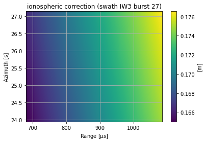
# correction = burst.get_correction('ionospheric')
#
# or equivalently
correction = burst.get_correction(s1etad.ECorrectionType.IONOSPHERIC, meter=True)
correction.keys()
[28]:
dict_keys(['x', 'unit', 'name'])
[29]:
az, rg = burst.get_burst_grid()
extent = [rg[0]*1e6, rg[-1]*1e6, az[0], az[-1]]

plt.figure()
plt.imshow(correction['x'], extent=extent, aspect='auto')
plt.xlabel('Range [$\mu s$]')
plt.ylabel('Azimuth [s]')
plt.grid()
plt.colorbar().set_label(f'[{correction["unit"]}]')
plt.title(f'{correction["name"]} correction (swath {burst.swath_id} burst {burst.burst_index})')
[29]:
Text(0.5, 1.0, 'ionospheric correction (swath IW3 burst 27)')
In alternative, the following (deprecated) methods are available:
get_tropospheric_correction(set_auto_mask=False, transpose=True, meter=False)
get_ionospheric_correction(set_auto_mask=False, transpose=True, meter=False)
get_geodetic_correction(set_auto_mask=False, transpose=True, meter=False)
get_bistatic_correction(set_auto_mask=False, transpose=True, meter=False)
get_doppler_correction(set_auto_mask=False, transpose=True, meter=False)
get_fmrate_correction(set_auto_mask=False, transpose=True, meter=False)
get_sum_correction(set_auto_mask=False, transpose=True, meter=False)
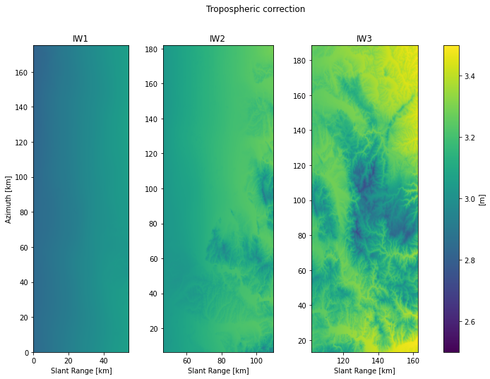
Retrieving merged corrections
The Sentinel1Etad and Sentinel1EtadSwath classes provides methods to retrieve a specific correction for multiple bursts merged together for easy reperesentation purposes.
NOTE: the current implementation uses a very simple argorithm that iterates over selected bursts and stitches correction data together. In overlapping regions new data simpy overwrite the old ones. This is an easy algorithm and perfectly correct for atmospheric and geodetic correction. It is, instead, sub-optimal for stsyem corrections (bi-static, Doppler, FM Rate) which have different values in overlapping regions.
[30]:
# First select you burst
first_time = parser.parse('2019-08-05T16:25:00.117898')
last_time =  parser.parse('2019-08-05T16:25:40.117899')

# query the catalogue for a subset of the swaths
product_name='S1B_IW_SLC__1SDV_20190805T162509_20190805T162536_017453_020D3A_AAAA.SAFE'
df = eta_.query_burst(first_time=first_time, last_time=last_time, product_name=product_name)
# df = df[df.bIndex != 13]   # exclude burst n. 13 (IW1)) to test extended selection capabilities
# df = df[df.bIndex != 17]   # exclude burst n. 17 (IW2)) to test extended selection capabilities
# df = df[df.bIndex != 15]   # exclude burst n. 17 (IW3)) to test extended selection capabilities
[31]:
# common variables
dy = eta_.grid_spacing['y']
dx = eta_.grid_sampling['x'] * constants.c / 2
nswaths = len(df.swathID.unique())
vg = eta_.grid_spacing['y'] / eta_.grid_sampling['y']
vmin = 2.5
vmax = 3.5
to_km = 1. / 1000
[32]:
# iterate on swath to get de-bursted data (selected burst merged together)
fig, ax = plt.subplots(nrows=1, ncols=nswaths, figsize=[13, 8]) # , sharey='row')
for six, swath_ in enumerate(eta_.iter_swaths(df)):
    merged_correction = swath_.merge_correction(ECorrectionType.TROPOSPHERIC,
                                                selection=df, meter=True)
    merged_correction_data = merged_correction['x']

    ysize, xsize = merged_correction_data.shape
    x0 = merged_correction['first_slant_range_time'] * constants.c / 2  # [m]
    y0 = merged_correction['first_azimuth_time'] * vg                   # [m]
    x_axis = (x0 + np.arange(xsize) * dx) * to_km
    y_axis = (y0 + np.arange(ysize) * dy) * to_km

    extent=[x_axis[0], x_axis[-1], y_axis[0], y_axis[-1]]
    im = ax[six].imshow(merged_correction_data, origin='lower', extent=extent,
                        vmin=vmin, vmax=vmax, aspect='equal')
    ax[six].set_title(swath_.swath_id)
    ax[six].set_xlabel('Slant Range [km]')

ax[0].set_ylabel('Azimuth [km]')

name = merged_correction['name']
unit = merged_correction['unit']

fig.suptitle(f'{name.title()} correction')
fig.colorbar(im, ax=ax[:].tolist(), label=f'[{unit}]')
[32]:
<matplotlib.colorbar.Colorbar at 0x7f8323d1ce10>
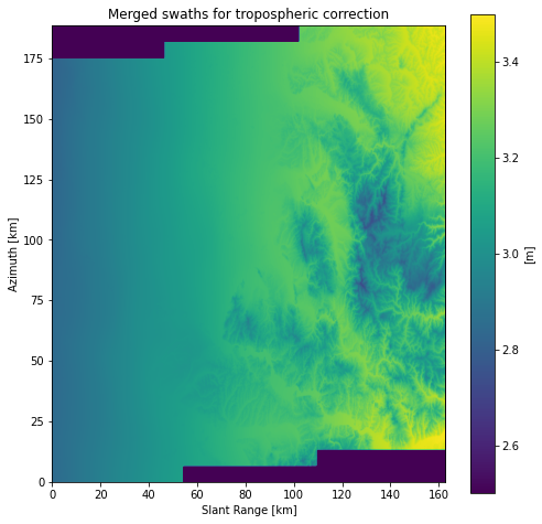
[33]:
# get merged swaths
fig, ax = plt.subplots(figsize=[8, 8])
merged_correction = eta_.merge_correction(ECorrectionType.TROPOSPHERIC,
                                          selection=df, meter=True)
merged_correction_data = merged_correction['x']

ysize, xsize = merged_correction_data.shape
x_axis = np.arange(xsize) * dx * to_km
y_axis = np.arange(ysize) * dy * to_km

extent=[x_axis[0], x_axis[-1], y_axis[0], y_axis[-1]]
im = ax.imshow(merged_correction_data, origin='lower', extent=extent,
               vmin=vmin, vmax=vmax, aspect='equal')

ax.set_xlabel('Slant Range [km]')
ax.set_ylabel('Azimuth [km]')

name = merged_correction['name']
unit = merged_correction['unit']

ax.set_title(f'Merged swaths for {name} correction')
fig.colorbar(im, ax=ax, label=f'[{unit}]')
[33]:
<matplotlib.colorbar.Colorbar at 0x7f8326d9f2d0>
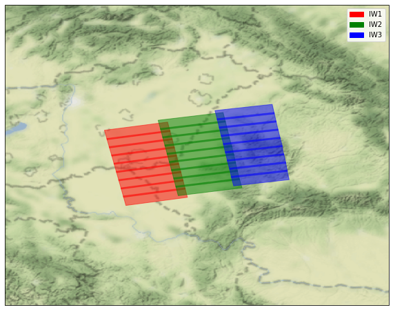
Use case 3 : Retrieving the footprints
[34]:
import cartopy.crs as ccrs
from matplotlib import patches as mpatches
from shapely.geometry import MultiPolygon

def tile_extent(poly, margin=2):
    bb = list(poly.bounds)
    bb [1:3] = bb [2:0:-1]
    bb2 = np.asarray(bb) + [-margin, margin, -margin, margin]
    return bb2

# get the footprints of the selected bursts
polys = eta_.get_footprint(swath_list=['IW1', 'IW2', 'IW3'])

fig = plt.figure(figsize=[10, 8])
ax = fig.add_subplot(1, 1, 1, projection=ccrs.PlateCarree())
ax.set_extent(tile_extent(MultiPolygon(polys)))

# Put a background image on for nice sea rendering.
OFFLINE = False
if OFFLINE:
    import cartopy.feature as cfeature
    ax.stock_img()
    ax.add_feature(cfeature.LAND)
    ax.add_feature(cfeature.COASTLINE)
else:
    import cartopy.io.img_tiles as cimgt
    # stamen_terrain = cimgt.Stamen('terrain-background')  # need cartopy >= 0.18
    stamen_terrain = cimgt.StamenTerrain()
    ax.add_image(stamen_terrain, 6)  # up to 10
    ax.coastlines()

# plot footprints of all selected burst
# ax.add_geometries(polys, crs=ccrs.PlateCarree(), alpha=0.8)

# get the footprints of each swath and plot them with different colors
items = []
for swath, color in zip(eta_, ['red', 'green', 'blue']):
    polys = swath.get_footprint()
    item = ax.add_geometries(polys, crs=ccrs.PlateCarree(), alpha=0.5,
                             color=color)
    items.append(item)

handles = [
    mpatches.Patch(color=color, label=label)
    for color, label in zip(['red', 'green', 'blue'], eta_.swath_list)
]
plt.legend(handles=handles)
/Users/valentino/anaconda3/envs/p37/lib/python3.7/site-packages/ipykernel_launcher.py:28: DeprecationWarning: The StamenTerrain class was deprecated in v0.17. Please use Stamen('terrain-background') instead.
[34]:
<matplotlib.legend.Legend at 0x7f830a2faf10>
[ ]: